Predicting NBA player retention
Authors: Alex Pandya, Peter Johnson, Andrew Newman, Ryan Moruzzi, and Collin Litterell
Background
The NBA is widely considered to be the best basketball league in the world, and has grown over its seven-decade existence into a multibillion-dollar industry. Central to this industry is the problem of roster construction, as team performance depends critically on selecting productive players for all 15 roster spots.
In this project, we aim to perform a novel analysis of NBA statistics, salary, and transaction data in order to determine whether or not a given player will be in the NBA in the next season (i.e., we predict NBA player retention). The resulting model has the potential to aid in the selection of players toward the end of the roster, which has long been one of the most challenging aspects of team construction.
Data collection and cleaning
Counting statistics data was collected from the official NBA site using an API and custom web scraping tools. Advanced statistics were collected from Kaggle. Transaction data and salary data were scraped from Basketball-Reference.com and hoopshype.com, respectively, using BeautifulSoup. The data was cleaned and missing data (e.g. missing salaries) were imputed. The data was split into a training set consisting of seasons 1990-91 through 2016-17 and a test set with seasons 2017-18 through 2022-23.
Exploratory data analysis
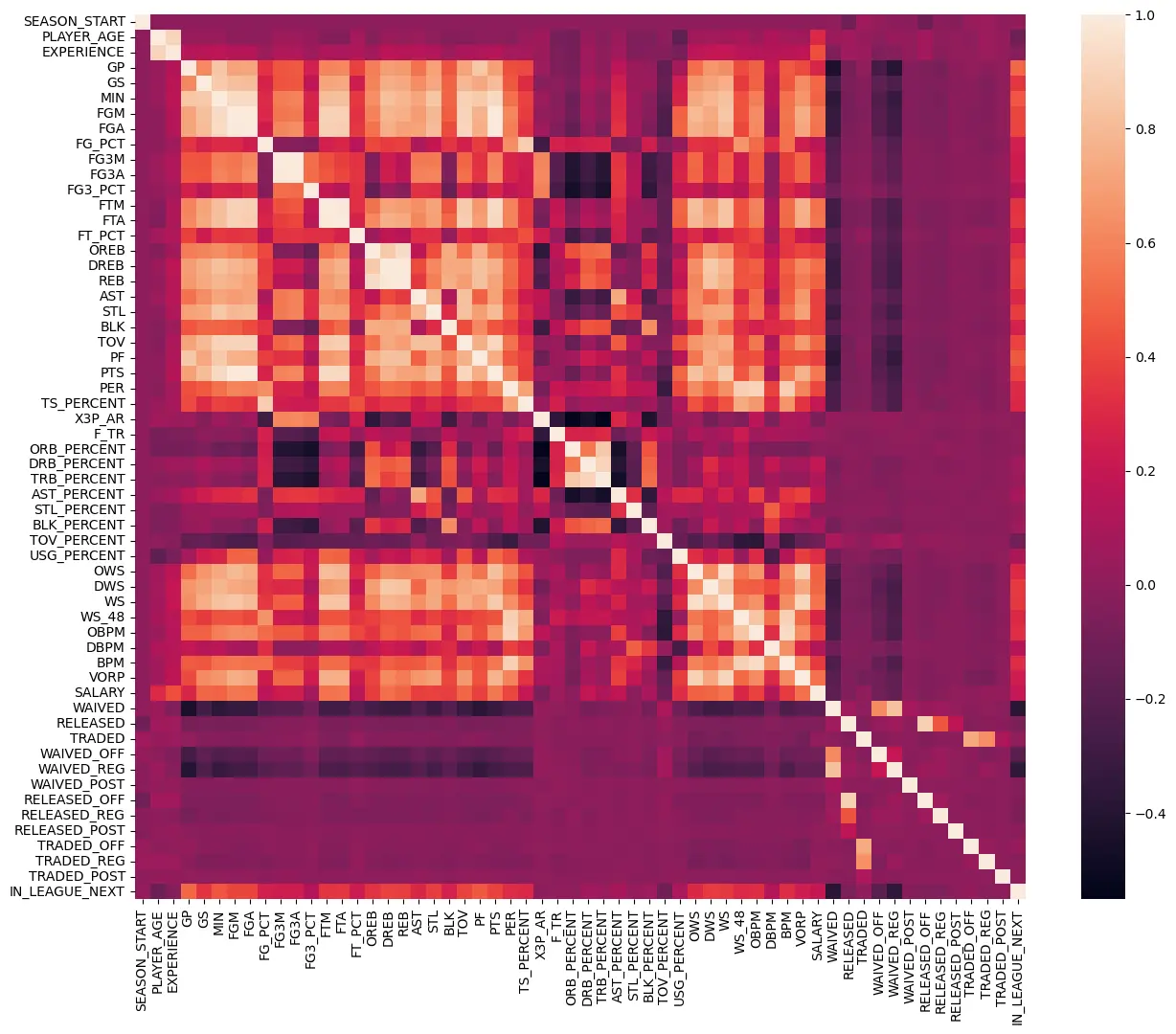
We initially aimed to predict player transactions (whether a given player would be traded/waived), but this proved challenging due to weak correlations between statistics and transaction data (magnitude ~0.05). We found appreciable correlations with whether a player stayed in the NBA in the following season (NBA player retention), however; see the plot below.

Modeling
Predicting NBA player retention in the following season is a classification problem with time series structure and imbalanced classes. We evaluated 10 models using walk-forward cross validation with the balanced accuracy score as our central metric. Most models were trained on an augmented training set produced using the Synthetic Minority Oversampling Technique (SMOTE) to balance classes. The table below summarizes the cross-validation performance of each model on the training dataset.
| Rank | Model | Balanced Accuracy | Precision | Recall (sensitivity) | NPV | Specificity | Hyperparameters |
|---|---|---|---|---|---|---|---|
| 1 | XGBoost Classifier | 0.8132 | 0.9455 | 0.8318 | 0.5244 | 0.7947 | n_estimators=350, learning_rate=0.005 |
| 2 | Random Forest Classifier | 0.8130 | 0.9498 | 0.8091 | 0.4990 | 0.8169 | max_depth=5, n_estimators=100 |
| 3 | Logistic Regression w. SMOTE | 0.8122 | 0.9593 | 0.7631 | 0.4582 | 0.8613 | C=0.0005 |
| 4 | AdaBoost Classifier | 0.8114 | 0.9555 | 0.7773 | 0.4703 | 0.8454 | learning_rate=0.1, n_estimators=100 |
| 5 | PCA + QDA | 0.8107 | 0.9560 | 0.7747 | 0.4671 | 0.8468 | pca__n_components=34, qda__reg_param=0.3 |
| 6 | LDA | 0.8091 | 0.9566 | 0.7683 | 0.4604 | 0.8498 | shrinkage=0.2 |
| 7 | Gaussian Naive Bayes | 0.7953 | 0.9658 | 0.6970 | 0.4075 | 0.8937 | var_smoothing=0.01 |
| 8 | PCA + KNN | 0.7932 | 0.9593 | 0.7172 | 0.4169 | 0.8692 | n_neighbors=28, n_components=28 |
| 9 | Decision Tree Classifier | 0.7917 | 0.9414 | 0.7962 | 0.4759 | 0.7871 | criterion=gini, max_depth=5 |
| 10 | Logistic Regression | 0.7370 | 0.8967 | 0.9430 | 0.6850 | 0.5310 | C=10.0 |
Calibration
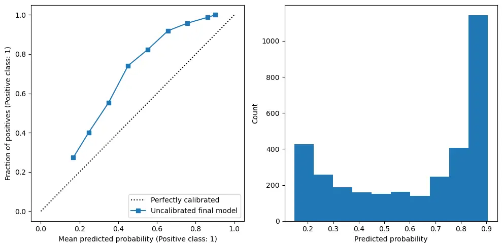
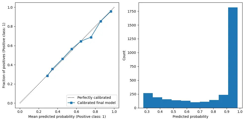
The best-performing model was calibrated using Platt scaling on a separate calibration set derived from the training data (but distinct from the data originally used to train the classifier). The uncalibrated model consistently underestimates the predicted probability of a player being retained; see the plot below.

Final model performance
The best-performing model on the training set, XGBoost with SMOTE-augmented training data, was evaluated on the unseen test set consisting of data from seasons starting in 2017-2022. The performance of the model on these seasons is summarized in the table below.
| Model | Balanced accuracy | Precision | Recall | NPV | Specificity | Uncalibrated Brier | Calibrated Brier |
|---|---|---|---|---|---|---|---|
| Baseline | 0.5000 | 0.7876 | 1.0000 | 0.0000 | 0.0000 | 0.2124 | 0.1678 |
| Final model | 0.8044 | 0.9455 | 0.7780 | 0.4985 | 0.8308 | 0.1463 | 0.1132 |
The final chosen model significantly outperforms the baseline (which just always chooses the majority class, “Retained”) in balanced accuracy, precision, NPV, specificity, and the uncalibrated/calibrated Brier scores.
Calibration of the final model (obtained using Platt scaling) is shown in the plot below.

Interactive summary site
An interactive summary site was created using the Python streamlit library, and can be found here.
Future Directions
To build on our existing model, some additional data that we could incorporate include:
- contract terms,
- injury information,
- G-League data,
- and salary cap and Collective Bargaining Agreement (CBA) data.
Additionally, we could expand our model of NBA players to incorporate other professional basketball leagues, for example the EuroLeague, and track movement across leagues. We could also expand the problem to focus on assigning probabilities that a player will be waived, traded, or not retained in the league at all, rather than pure classification.